
计划在这篇博客里调研并粗略地学习一下到目前为止比较有影响力的AI Infra工作(类似Survey),并慢慢补充丰富。Anyway,迈出行动的第一步最难。
Model Parameters
Parameter Estimation
1B = 1 Billion = 十亿
假设模型层数为$N$,隐藏层维度为$H$,接下来考虑一层Transformer层的参数量估算:
- 自注意力层:(不需要考虑MHA的情况,因为多头concat起来的为度就等于隐藏层维度)需要注意的是这里包括一次注意力计算和一次线性映射,因此涉及四个可训练参数$W_Q$、$W_K$、$W_V$和$W_O$,因此注意力层的可训练参数量为$4H^2 + 4H$。
- 前馈网络层:FFN层包括一次线性升维和一次线性降维,设计两个可训练参数$W_{1}$和$W_{2}$,可训练参数量为$(H\times 4H + 4H) + (4H \times H + H) = 8H^{2} + 5H$。
- 残差连接和层归一化:Add & Norm层(主要是LN层)涉及两个可训练向量参数$\alpha$和$b$,即2H。
综上,一层Transformer层由一层Attention层、一层FFN层和两层Add & Norm层组成,可训练参数量为$12H^{2} + 13H$,可以近似为$12H^{2}$。
Computation Estimation
AxB和BxC的矩阵相乘,每个输出元素需要进行$n$次乘法和$n-1$次加法,$\approx 2n FLOPs$;整个矩阵共有AxC个输出元素,因此总$FLOPs \approx 2ABC$,可以近似为$ABC$。因此估算参数时,主要关注矩阵乘或向量矩阵乘的维度即可。注意$W_{Q/K/V}$的维度是$HxH$,而$Q/K/V$的维度是$LxH$。
接下来估算计算量,由于LayerNorm、Dropout等计算量较小,暂时不考虑。设模型层数为$N$,隐藏层维度为$H$,批量大小为$B$,序列长度为$L$:
- 自注意力层
(LHxHH=LH)线性投影QKV:每个投影是$H\times H$,应用于每个token就是$BLH^{2}$,总共3个矩阵,因此$FLOPs=3BLH^{2}$
(LHxHL=LL)Attention Score ($QK^{T}$):每个token对应一个$L\times L$的注意力矩阵,需要做$H$次乘加,约为$BHL^{2}$
(——————)Softmax和Scaling:Softmax涉及取指、求和、逐元素除和、数值稳定的计算,这里只能估计为$xBL^{2}$,相比SDPA可忽略不计
(LLxLH=LH)Attention Output与V相乘:显然是$BHL^{2}$
(LHxHH=LH)输出线性层$W_{O}$:显然是$BLH^{2}$
因此,自注意力层的总FLOPs:
$$\approx (3BLH^{2})+(2BHL^{2})+(BLH^{2})=4BLH^{2}+2BHL^{2}$$- 前馈网络层:
升维($H$->$4H$):$FLOPs=BLH(4H)$
降维($4H$->$H$):$FLOPs=BL(4H)H$
(当然还有GeLU激活,不过是线性的计算量,可以忽略不计)因此,FFN层的总Flops:
$$\approx 8BLH^{2}$$综上,$Total\ FLOPs \approx 12BLH^{2} + 2BHL^{2}$$。(理论上应该再乘以2)
Memory Estimation
Inference Optimization
KV Cache OPtimization
KV Cache
KV (Key-Value) Cache是一种在自回归模型(如Decoder of Transformer)中常用的推理加速技术,通过在推理的注意力机制计算过程中缓存已计算过的$Key$和$Value$,减少重复的$K$、$V$与权重矩阵的projection计算。
$$Attention(Q, K, V)=softmax(\frac{QK^{T}}{\sqrt[]{d_{k}} })V$$为什么可以缓存$K$和$V$?由于Casual Mask机制,当模型推理时当前token不需要与之后的token进行Attention计算,因此在计算第$t$个token的$Attention_{t}$时,只需要$Q_{0:t}$、$K_{0:t}$和$V_{0:t}$。而Decoder中的$Q$需要token在embedding后通过$W_q$投影,但$K_{0:t-1}$与$V_{0:t-1}$来自Encoder中,且在计算$Attention_{0:t-1}$时已被计算过,因此可以通过缓存已被计算过的历史$K$与$V$来节省这部分计算。
接下来参考知乎@看图学的公式推导,
计算第一个token时的Attention:
$$ Attention(Q, K, V) = softmax(\frac{Q_{1}K_{1}^{T}}{\sqrt[]{d}})V_{1} $$计算第二个token时的Attention(矩阵第二行对应$Attention_{2}$),$softmax(\frac{Q_{1}K_{2}}{\sqrt d})$项被mask掉了:
$$ Attention(Q, K, V) = softmax(\frac{Q_{2}[K_{1}, K_{2}]^{T}}{\sqrt[]{d}})[V_{1}, V_{2}] \newline = \begin{pmatrix} softmax(\frac{Q_{1}K_{1}^{T}}{\sqrt d}) & softmax(-\infty )\\ softmax(\frac{Q_{2}K_{1}^{T}}{\sqrt d}) & softmax(\frac{Q_{2}K_{2}^{T}}{\sqrt d}) \end{pmatrix}[V_{1}, V_{2}] \newline =\begin{pmatrix} softmax(\frac{Q_{1}K_{1}^{T}}{\sqrt d})V_{1} + 0 \times V_{2} \\ softmax(\frac{Q_{2}K_{1}^{T}}{\sqrt d})V_{1} + softmax(\frac{Q_{2}K_{2}^{T}}{\sqrt d})V_{2} \end{pmatrix} $$以此类推,Attention矩阵的严格上三角部分都被mask掉了,因此计算第$t$个token的$Attention_{t}$时与$Q_{1:t-1}$无关:
$$ Attention_{1} = softmax(\frac{Q_{1}K_{1}^{T}}{\sqrt[]{d}})V_{1} \newline Attention_{2} = softmax(\frac{Q_{1}[K_{1}, K_{2}]^{T}}{\sqrt[]{d}})[V_{1}, V_{2}] \newline ... \newline Attention_{t} = softmax(\frac{Q_{t}K_{1:t}^{T}}{\sqrt[]{d}})V_{1:t} $$源码实现参考Huggingface的GPT2推理实现,KV Cache的逻辑核心思路如下:
对于
Cross Attention,$Q$来自decoder的当前token,$KV$来自encoder的全部输出。因此$KV$通常不变,只需生成一次并缓存。对于
Self Attention,$QKV$都来自decoder的当前token,因为decoder需要看过去所有的token,因此前面token的$KV$都需要缓存
看源码好难——
| |
同时,KV Cache在减少重复$KV$计算的同时会引入大量的Memory开销,可以粗略计算一下KV Cache的显存占用:
$$ Memory = 2 \times batch\_size \times seq\_len \times num\_layers \times num\_heads \times head\_dims \times dtype\_size $$MQA
Multi-Query Attention (MQA)是Google在2019年于《Fast Transformer Decoding: One Write-Head is All You Need》提出的一种高效注意力机制,旨在减少推理过程中的计算和内存开销。与传统MHA不同,MQA保留多个Query头,但所有注意力头共享同一组Key和Value,这种结构显著减少了KV Cache的Memory开销,同时保持了MHA相近的性能表现。
下面是基于PyTorch的一个简单实现(还没实现Casual Mask):
| |
GQA
Grouped-Query Attention (GQA)Google与在023年于GQA: Training Generalized Multi-Query Transformer Models from Multi-Head Checkpoints提出的一种介于MHA和MQA之间的注意力机制,让多个Query头共享同一组Key和Value,旨在保留部分表达能力的同时大幅减少计算和内存开销。

Overview of grouped-query method
源码上,只在Huggingface的仓库里找到了sdpa_attention_paged_forward的实现,看上去挺GQA的。
核心思路是:
先用
repeat_kv将KV head复制num_attention_heads // num_key_value_heads次(从(B, num_key_value_heads, L, D)到(B, num_attention_heads, L, D))支持KV Cache的SDPA
Preliminaries (FlashAttention)
FlashAttention由Tri Dao等在2022年于《FlashAttention: Fast and Memory-Efficient Exact Attention with IO-Awareness》提出,并在2023年于《FlashAttention-2: Faster Attention with Better Parallelism and Work Partitioning 》提出v2版本,2024年于《FlashAttention-3: Fast and Accurate Attention with Asynchrony and Low-precision》提出v3版本。
Online Softmax
Naive Softmax涉及两次read(遍历求sum和逐元素除sum(exp))和一次write(结果写回),数学公式如下:
$$softmax(x_{i}) = \frac{e^{x_{i}}}{\Sigma _{j=1}^{n}e^{x_{j}}}$$如果$x$太大,$e^x$会上溢,而safe softmax解决了这一问题。
Safe Softmax涉及三次read(还需要遍历一次减去max)和一次write,目的是为了避免数值溢出,数学公式如下:
$$softmax(x_{i}) = \frac{e^{x_{i} - max(x)}}{\Sigma _{j=1}^{n}e^{x_{j} - max(x)}}$$但是需要多次遍历数据,性能较差,而online softmax解决了这一问题。
Online Softmax只需要两次read(遍历一次x并维护最大值和归一化因子)和一次write,核心思路如下:
在线维护变量($m_t$,当前前$t$个元素的最大值;$d_t$,当前前$t$个元素的归一化因子)
初始化
$m_0=-\infty, d_0=0$
遍历并维护变量
更新最大值:
$m_t=max(m_{t-1}, x_t)$
更新归一化因子(递推)【难点】:
$d_t=d_{t-1}\cdot e^{m_{t-1}-m_t}+e^{x_t - m_t}(=\Sigma_{j=1}^{t-1}e^{x_j-m_{t-1}}\cdot e^{m_{t-1}-m_t}+e^{x_t - m_t})$
这里的公式推导非常巧妙,应用了同底指数相乘等于两个指数幂相加,论文的推导如下,$d_{t}$代表前$t$个数与最大值(局部,即$m_t$)之差的指数和:
$$d_t = d_{t-1}\times e^{m_{t-1}-m_t} + e^{x_t-m_t} \newline =(\Sigma_{j=1}^{t-1}e^{x_j-m_{t-1}}) \times e^{m_{t-1}-m_t} + e^{x_t-m_t} \newline = \Sigma_{j=1}^{t-1}e^{x_j-m_t}+e^{x_t-m_t} \newline = \Sigma_{j=1}^{t}e^{x_j-m_t}$$可以这么理解:每次更新归一化因子时,都乘以了$e^{m_{t-1} - m_{t}}$,那么最后这个因子会是$e^{0-m_{global}}$,正是分母$e^{x_{t}-m_{global}}$的一部分,如此巧妙地将全局最大值保留到了遍历结束,而且在递推中的每一步都纠正了之前的局部最大值
online softmax的伪代码如下,实现上还是比较简单的:
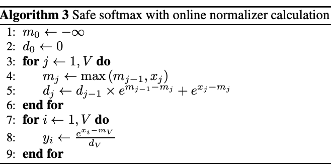
Pseudocode of Online Softmax
参考@TaurusMoon的实现写了C++的online softmax kernel:
| |
GPU Memory Architecture
显存/高带宽内存(HBM, High Bandwidth Memory)是封装在GPU Core外的DRAM(动态存储,需要周期性刷新),通过超宽总线连接GPU Core,大容量的同时延迟也相对较大。
静态内存(SRAM, Static Random Access Memory)**是封装在GPU Core内部的SRAM(静态存储),如Register、Shared Memory、L1/L2 Cache。
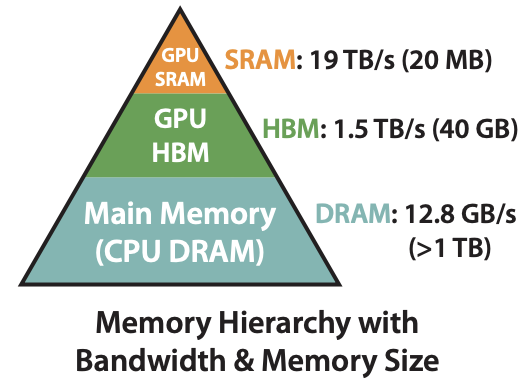
Memory/Bandwidth Architcture of A100
Operator
算子主要可以分为两类:
计算受限型:如GEMM等
内存受限型:主要是element-wise类(如Activation、Dropout、Maskibg等)和reduction类(如Sum、Softmax、LayerNorm等)
FlashAttention
FlashAttention-v1
Transformer的核心计算是Attention,朴素的Attention计算步骤如下,其中一般$N \gg d$,复杂度是$N^2$,在长序列频繁读写(5read & 3 write)大矩阵时非常依赖HBM:
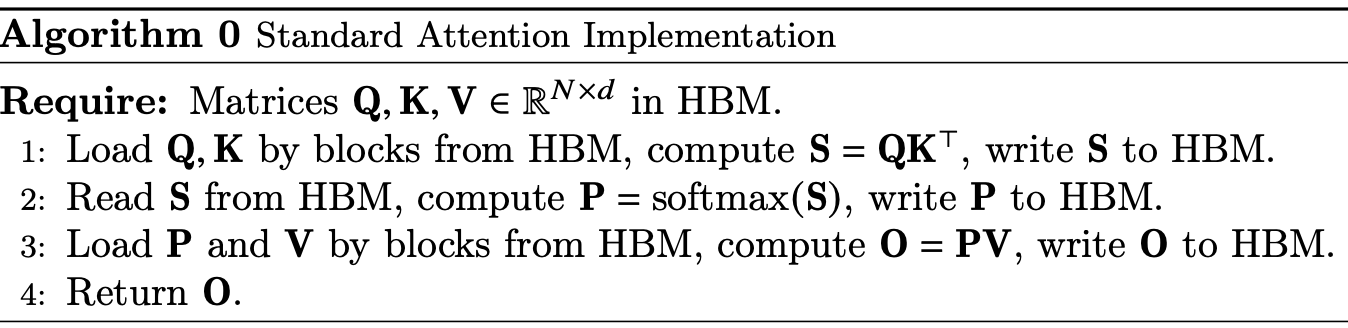
Standard Attention Implementation
FlashAttention的核心思路就是提高Attention算子的SRAM利用率(将输入的QKV矩阵从HBM加载到SRAM中计算),减少HBM访存。
- Tiling
常规的row-wise softmax不适合分块的算法,因此这里需要使用online softmax,在分块后的范围内,片上计算max和rowsum,并在通信后计算全局的max和scale factor。
- Recomputation
在反向传播的优化,计算梯度需要用到QK计算的attention score ($S$)和softmax后的attention score ($P$)。FlashAttention通过存储Attention的输出结果($O$)和归一化统计量$(m, l)$来快速计算$S$和$P$,避免了用$QKV$的重复计算。
- Kernel Fusion
很常见的优化,减少了多余的HBM写回和重新加载。
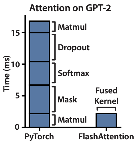
PyTorch vs. FlashAttention on GPT-2
总结一下,FlashAttention可以让计算提速2-4倍,节约10倍以上内存(主要是边存变算,不用存储复杂度为$N^2$的$QKV$,转而存储复杂度为$Nd$的输出结果和统计量)。
Training Optimization
Parallel Computting (on Data)
DP
数据并行(DP, Data Parallel):模型副本在每个GPU上各自独立地前向传播,梯度会聚合(AllReduce)到主GPU进行参数更新。缺点是非跨进程,只支持单机多卡;梯度聚合会发生在主设备,导致通信瓶颈和负载不均衡。
实现上较为简单:
| |
不过PyTorch建议多卡并行的时候使用DPP,即使只有一个节点(DP的性能较DDP更差,因为主卡负载很不均衡,单进程多线程环境下设计GIL竞争,且可扩展性不如DDP),源码实现见这里,更加底层的Operator在torch.nn.parallel.scatter_gather/_functions/comm下(如scatter、gather等)。
DDP
分布式数据并行(DDP, Distributed Data Parallel):每个进程对应一个GPU,每个GPU上都有模型副本,梯度通过AllReduce同步,每个金层都参与参数更新(每个GPU独立进行前向、计算loss、计算梯度,并在AllReduce后通过平均梯度更新)。
实现上可以通过手动设置并行(多个terminal设置RANK、WORLD_SIZE、MASTER_ADDR、MASTER_PORT等环境变量并启动脚本)或用torchrun自动管理环境变量(torchrun --nproc_per_node=... <script>):
| |
源码参考这里。DDP可以使用高效的通信后端(如NCCL),没有主从瓶颈(支持单机多卡/多机多卡),还是非常实用的。
FSDP
全分片数据并行(FSDP, Fully Sharded Data Parallel):模型权重按参数维度切分到多个GPU上(shard),前向传播时重新聚合参数(gather),反向传播后再切分(reshard),大幅减少显存占用,主要通过torch.nn.distributed.fsdp.FullyShardedDataParallel来实现,源码参考这里。
本质上FSDP还是数据并行,知识参数分别有点模型并行的味道
Parallel Computting (on Model)

Existing parallelism for distributed training (sorry我没找到图片来源)
TP
张量并行(TP, Tensor Parallel):是一种层内并行(Intra-Layer Parallelism)策略,将模型中的一个层(如MLP层、Attention层)的内部计算划分到多个设备上,多个设备共同完成该层前向和反向传播。这么做可以突破显存的限制,但是会对延迟较敏感。
- Column-wise Parallelism (切列,维度完整)
- Row-wise Parallelism (切行)
PP
流水线并行(PP, Pipeline Parallel):是一种层间并行(Inter-Layer Parallelism)策略,将模型按顺序划分为多个stage,不同GPU执行不同的stage,多个micro-batch以流水线方式通过模型。
支持极大模型(层数多),显存需求分布在各stage,且跨GPU通信压力小;但是存在pipeline bubble(起始阶段GPU空闲,影响吞吐)
Quantization
Precision Formats
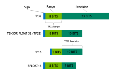
TF32 strikes a balance that delivers performance with range and accuracy
IEEE 754标准中浮点数由三部分组成:S符号位、E指数位、M尾数位,接下来介绍各种精度格式:
FP32标准的IEEE 754单精度浮点格式,1位符号位+8位指数位+23位位数(下文用[S, E, M]来表示),精度较高,适用于所有主流硬件(CPU、GPU、TPU等)TP32NVIDIA在Ampere架构引入的混合格式,[1, 8, 10],截断了尾数位(减少乘加复杂度),支持Tensor Core优化,精度介于FP32和FP16之间,常在训练时作为FP32替换FP1616-bit半精度浮点数,[1, 5, 10]BF16Google TPU推出的Brain Float 16,[1, 8, 7],常用于混合精度训练FP8[1, 4, 3]或[1, 5, 2],需要Hopper架构GPU支持INT88-bit整型FP4[1, 2, 1]
Reference
LM(20):漫谈 KV Cache 优化方法,深度理解 StreamingLLM
Fast Transformer Decoding: One Write-Head is All You Need
GQA: Training Generalized Multi-Query Transformer Models from Multi-Head Checkpoints
FlashAttention: Fast and Memory-Efficient Exact Attention with IO-Awareness
FlashAttention-2: Faster Attention with Better Parallelism and Work Partitioning
FlashAttention-3: Fast and Accurate Attention with Asynchrony and Low-precision