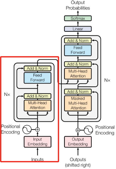
BERT Architecture Total Summary BERT的模型架构完全基于Transformer架构的编码器(Encoder)堆叠(原文使用12层或24层Transformer Layer),每个Encoder包括多头自注意力机制 (MHA,Multi-Head Self-Attention,支持双向上下文理解)、前馈神经网络 (FFN,Feed-Forward Network,对注意力输出进行非线性变换),参差连接和层归一化 (Add & Norm,提升训练稳定性)。
Transformer Model Architecture A Simple Demo 这里以一个Huggingface发布的用于英文句子情感二分类的蒸馏BERTDistilBERT (distilbert-base-uncased-finetuned-sst-2-english) 66M 为例,使用transformers库实现加载并推理。
1
huggingface-cli download distilbert/distilbert-base-uncased-finetuned-sst-2-english --local-dir distilbert-base-uncased-finetuned-sst-2-english
下载模型后,即可通过AutoTokenizer和AutoModelForSequenceClassification导入模型。
 1
 2
 3
 4
 5
 6
 7
 8
 9
10
11
12
13
14
15
16
17
18
19
20
21
22
import torch.nn.functional as F
from transformers import AutoTokenizer , AutoModelForSequenceClassification
# 加载tokenizer和model
model_name = '/path/to/bert-model'
tokenizer = AutoTokenizer . from_pretrained ( model_name )
model = AutoModelForSequenceClassification . from_pretrained ( model_name )
# sentence -> tokens
test_sentences = [ 'today is not that bad' , 'today is so bad' ]
batch_input = tokenizer ( test_sentences , padding = True , truncation = True , return_tensors = 'pt' )
# inference
with torch . no_grad ():
outputs = model ( ** batch_input ) # 解包tokens -> inference result
print ( "outputs" , outputs )
scores = F . softmax ( outputs . logits , dim = 1 ) # 对logits(预测分数)对每一行(类别)进行softmax
print ( "scores" , scores )
labels = torch . argmax ( scores , dim = 1 ) # 沿类别维度获取最大值索引
labels = [ model . config . id2label [ id . item ()] for id in labels ] # 0->LABEL_0, 1->LABEL_1
print ( "labels" , labels )
即可得到以下推理结果:
1
2
3
4
5
outputs SequenceClassifierOutput( loss = None, logits = tensor([[ -3.4620, 3.6118] ,
[ 4.7508, -3.7899]]) , hidden_states = None, attentions = None)
scores tensor([[ 8.4632e-04, 9.9915e-01] ,
[ 9.9980e-01, 1.9531e-04]])
labels [ 'POSITIVE' , 'NEGATIVE' ]
关于with torch.no_grad()和param.requires_grad=False的区别:
接下来需要对一些细节进行补充。
model.config model.config用于存储模型架构和训练配置。
 1
 2
 3
 4
 5
 6
 7
 8
 9
10
11
12
13
14
15
16
17
18
19
20
21
22
23
24
25
26
27
28
29
30
31
32
33
DistilBertConfig {
  "activation": "gelu",
  "architectures": [
    "DistilBertForSequenceClassification"
  ],
  "attention_dropout": 0.1,
  "dim": 768,
  "dropout": 0.1,
  "finetuning_task": "sst-2",
  "hidden_dim": 3072,
  "id2label": {
    "0": "NEGATIVE",
    "1": "POSITIVE"
  },
  "initializer_range": 0.02,
  "label2id": {
    "NEGATIVE": 0,
    "POSITIVE": 1
  },
  "max_position_embeddings": 512,
  "model_type": "distilbert",
  "n_heads": 12,
  "n_layers": 6,
  "output_past": true,
  "pad_token_id": 0,
  "qa_dropout": 0.1,
  "seq_classif_dropout": 0.2,
  "sinusoidal_pos_embds": false,
  "tie_weights_": true,
  "torch_dtype": "float32",
  "transformers_version": "4.52.3",
  "vocab_size": 30522
}
Rules on Tokenizer 调用tokenizer即调用tokenizer.__call__或tokenizer.encoder(不完全等价,encoder默认不返回attention_mask),将返回含有input_ids和attention_mask的输入字典(inputs_ids和attention_mask长度一致)。(具体返回什么视模型具体需要而定)
tokenizer.encoder的调用分为两步,先分词,再编码,所以等价于先调用tokenizer.tokenize再调用tokenizer.convert_tokens_to_ids。
在句子对编码时,使用tokenizer.encode_plus,在返回字典中除了inputs_ids和attention_mask,还会返回token_type_ids$\in {0, 1}$用于标记第一句话和第二句话。在tokens中,会用[SEQ]分割。
 1
 2
 3
 4
 5
 6
 7
 8
 9
10
# 编码
print ( tokenizer ( test_sentences [ 0 ]))
# tokenizer.encode = tokenizer.tokenize + tokenizer.convert_tokens_to_ids
print ( tokenizer . encode ( test_sentences [ 0 ],))
## tokenize
print ( tokenizer . tokenize ( test_sentences [ 0 ]))
## convert_tokens_to_ids
print ( tokenizer . convert_tokens_to_ids ( tokenizer . tokenize ( test_sentences [ 0 ])))
# 解码
print ( tokenizer . decode ([ 101 , 2651 , 2003 , 2025 , 2008 , 2919 , 102 ]))
可以得到以下结果:
1
2
3
4
5
6
7
8
9
# 编码
{ 'input_ids' : [ 101, 2651, 2003, 2025, 2008, 2919, 102] , 'attention_mask' : [ 1, 1, 1, 1, 1, 1, 1]}
[ 101, 2651, 2003, 2025, 2008, 2919, 102]
## tokenize
[ 'today' , 'is' , 'not' , 'that' , 'bad' ]
## convert_tokens_to_ids
[ 2651, 2003, 2025, 2008, 2919]
# 解码
[ CLS] today is not that bad [ SEP]
tokenizer是根据tokenizer.vocab为依据进行编码的,以下是特殊token表(可以通过tokenizer.special_tokens_map或直接tokenizer查看),tokenizer会尽量避免将词分为[UNK](存在5828个##开头的后缀子词)。
1
2
3
4
5
{'unk_token': '[UNK]',      # 100
 'sep_token': '[SEP]',      # 102
 'pad_token': '[PAD]',      # 0
 'cls_token': '[CLS]',      # 101
 'mask_token': '[MASK]'     # 103}
Parameter 这里以Google发布的google-bert/bert-base-uncased (12层BertLayer)为例。
通过model可以看到BERT的架构如下:
Embedding 由word embeddings、position embeddings和token type embedding三部分组成
Encoder 由12层BertLayer组成,每层BertLayer都由一次Self Attention和一次FFN组成
Pooler 全连接层
Output (optional)作为下游任务的输出层
 1
 2
 3
 4
 5
 6
 7
 8
 9
10
11
12
13
14
15
16
17
18
19
20
21
22
23
24
25
26
27
28
29
30
31
32
33
34
35
36
37
38
39
40
41
BertModel(
  (embeddings): BertEmbeddings(
    (word_embeddings): Embedding(30522, 768, padding_idx=0)
    (position_embeddings): Embedding(512, 768)
    (token_type_embeddings): Embedding(2, 768)
    (LayerNorm): LayerNorm((768,), eps=1e-12, elementwise_affine=True)
    (dropout): Dropout(p=0.1, inplace=False)
  )
  (encoder): BertEncoder(
    (layer): ModuleList(
      (0-11): 12 x BertLayer(
        (attention): BertAttention(
          (self): BertSdpaSelfAttention(
            (query): Linear(in_features=768, out_features=768, bias=True)
            (key): Linear(in_features=768, out_features=768, bias=True)
            (value): Linear(in_features=768, out_features=768, bias=True)
            (dropout): Dropout(p=0.1, inplace=False)
          )
          (output): BertSelfOutput(
            (dense): Linear(in_features=768, out_features=768, bias=True)
            (LayerNorm): LayerNorm((768,), eps=1e-12, elementwise_affine=True)
            (dropout): Dropout(p=0.1, inplace=False)
          )
        )
        (intermediate): BertIntermediate(
          (dense): Linear(in_features=768, out_features=3072, bias=True)
          (intermediate_act_fn): GELUActivation()
        )
        (output): BertOutput(
          (dense): Linear(in_features=3072, out_features=768, bias=True)
          (LayerNorm): LayerNorm((768,), eps=1e-12, elementwise_affine=True)
          (dropout): Dropout(p=0.1, inplace=False)
        )
      )
    )
  )
  (pooler): BertPooler(
    (dense): Linear(in_features=768, out_features=768, bias=True)
    (activation): Tanh()
  )
)
可以用以下代码计算每一部分的参数量:
 1
 2
 3
 4
 5
 6
 7
 8
 9
10
11
12
13
14
15
16
17
18
19
20
21
22
23
24
25
26
total_params = 0
total_learnable_params = 0
total_embedding_params = 0
total_encoder_params = 0
total_pooler_params = 0
for name , param in model . named_parameters ():
# print(name, '->', param.shape, '->', param.numel())
# 加上`if param.requires_grad:`可以计算可学习参数量
if 'embedding' in name :
total_embedding_params += param . numel ()
if 'encoder' in name :
total_encoder_params += param . numel ()
if 'pooler' in name :
total_pooler_params += param . numel ()
if param . requires_grad :
total_learnable_params += param . numel ()
total_params += param . numel ()
params = [
( "total_embedding_params" , total_embedding_params ),
( "total_encoder_params" , total_encoder_params ),
( "total_pooler_params" , total_pooler_params )
]
for name , param in params :
percentage = ( param / total_params ) * 100
print ( f " { name } : { percentage : .2f } %, { param } " )
得到输出结果:
1
2
3
total_embedding_params: 21.77 %, 23837184
total_encoder_params: 77.69 %, 85054464
total_pooler_params: 0.54 %, 590592
Output 在outputs = model(**input)后调用type(outputs)可以发现Bert的输出类型是transformers.modeling_outputs.BaseModelOutputWithPoolingAndCrossAttentions。参考Huggingface-BERT文档 ,默认情况下长度为2(last_hidden_state和pooler_output)。当定义模型时指定output_hidden_states=True时,还会返回hidden_state,其他参数类似。
output[0] (last_hidden_state), shape = (batch_size, seq_len, hidden_size)
output[1] (pooler_output), shape = (batch_size, hidden_size)
最终隐藏状态(classification token, [CLS]的输出)
output[2] (hidden_states), tuple , embedding layer和每个layer的输出(1+12), shape = 13 * (batch_size, seq_len, hidden_size) 如model.embeddings(input['input_ids'], input['token_type_ids']) == outputs[2][0]表示Embedding层的输出。
Embedding 上文提到,BERT的Embedding层由word embeddings、position embeddings和token type embedding三部分组成,以下代码实现了简单的Embedding层:
 1
 2
 3
 4
 5
 6
 7
 8
 9
10
11
12
13
14
15
16
17
18
19
20
21
22
23
24
25
from transformers import BertTokenizer , BertModel
tokenizer = BertTokenizer . from_pretrained ( "bert-base-uncased" )
model = BertModel . from_pretrained ( "bert-base-uncased" )
input = tokenizer ( sentence , return_tensors = 'pt' ) # {input_ids, token_type_ids, attention_mask}
input_ids = input [ 'input_ids' ] # shape = (batch_size, token_len)
token_type_ids = input [ 'token_type_ids' ] # shape = (batch_size, token_len)
pos_ids = torch . arange ( input_ids . shape [ 1 ]) # shape = (token_len)
# 1. Word Embedding
word_embed = model . embeddings . word_embeddings ( input_ids ) # shape = (batch_size, token_len, embedding_size=768)
# 2. Token Type Embedding
tok_embed = model . embeddings . token_type_embeddings ( token_type_ids ) # shape = (batch_size, token_len, embedding_size=768)
# 3. Position Embedding
pos_embed = model . embeddings . position_embeddings ( pos_ids ) # shape = (token_len, embedding_size=768)
# **Input Embedding**
input_embed = word_embed + tok_embed + pos_embed . unsqueeze ( 0 ) # 也可以不unsqueeze, 会broadcast的
# 后处理
embed = model . embeddings . LayerNorm ( input_embed )
embed = model . embeddings . dropout ( embed )
Self-Attention $$Attention(Q, K, V)=softmax(\frac{QK^{T}}{\sqrt[]{d_{k}} })V$$接下来是从Embedding层输出到Multi-Head Self-Attention (MHA)的代码实现(first head):
 1
 2
 3
 4
 5
 6
 7
 8
 9
10
11
att_head_size = int ( model . config . hidden_size / model . config . num_attention_heads ) # 768 / 12 = 64
emb_output = model . embeddings ( input [ 'input_ids' ], input [ 'token_type_ids' ]) # shape = (batch_size, seq_len, embedding_dim)
# emb_output[0].shape = (seq_len, embedding_dim)
## Why Transpose? 因为PyTorch中的Linear里就是x@A^T(左乘转置)
Q_first_head_first_layer = emb_output [ 0 ] @ model . encoder . layer [ 0 ] . attention . self . query . weight . T [:, : att_head_size ] + model . encoder . layer [ 0 ] . attention . self . query . bias [: att_head_size ]
K_first_head_first_layer = emb_output [ 0 ] @ model . encoder . layer [ 0 ] . attention . self . key . weight . T [:, : att_head_size ] + model . encoder . layer [ 0 ] . attention . self . key . bias [: att_head_size ]
# (seq_len, att_head_size) @ (seq_len, att_head_size).T -> (seq_len, seq_len)
attn_scores = torch . nn . Softmax ( dim =- 1 )( Q_first_head_first_layer @ K_first_head_first_layer . T ) / math . sqrt ( att_head_size )
V_first_head_first_layer = emb_output [ 0 ] @ model . encoder . layer [ 0 ] . attention . self . value . weight . T [:, : att_head_size ] + model . encoder . layer [ 0 ] . attention . self . value . bias [: att_head_size ]
attn_emb = attn_scores @ V_first_head_first_layer # shape = (seq_len, att_head_size)
接下来是关于MHA的公式推导,定义$E$为Embedding层的输出$q$、$k$、$v$分别为同一token对应的query、key、value,$W_q$、$W_k$、$W_v$分别为同一token的权重,$Q$、$K$、$V$分别为整个序列的query、key、value,$W_Q$、$W_K$、$W_V$分别为整个序列的权重。这里省略bias项。
先从某一token出发,$T$表示序列长度,$d_e$表示Embedding层维度,$d_q$、$d_k$、$d_v$分别表示q、k、v的维度,$E \in \mathbb{R}^{T \times d_e}$,那么:
$$E \cdot W_q = q \in \mathbb{R}^{T \times d_q}$$$$E \cdot W_k = k \in \mathbb{R}^{T \times d_k}$$$$E \cdot W_v = v \in \mathbb{R}^{T \times d_v}$$其中$d_q == d_k$,因为后续需要计算$q \cdot k^{T}$,$d_v$则没有要求:
$$Attention\ Score = Softmax(\frac{q \cdot k^{T}}{\sqrt{d_k}}) \in \mathbb{R}^{T \times T}$$$$Attention\ Output = Softmax(\frac{q \cdot k^{T}}{\sqrt{d_k}}) \cdot v \in \mathbb{R}^{T \times d_v}$$接下来定义Attention头数为$n$,将单头的情况拓展到多头:
\[
\left[
\begin{array}{c|c|c|c}
E\cdot W_{q_1} & E\cdot W_{q_2} & ... & E\cdot W_{q_n} \\
\end{array}
\right]=E\cdot \left[
\begin{array}{c|c|c|c}
W_{q_1} & W_{q_2} & ... & W_{q_n} \\
\end{array}
\right]=E\cdot W_Q=Q \in \mathbb{R}^{T \times n\cdot d_q}
\]\[
\left[
\begin{array}{c|c|c|c}
E\cdot W_{k_1} & E\cdot W_{k_2} & ... & E\cdot W_{k_n} \\
\end{array}
\right]=E\cdot \left[
\begin{array}{c|c|c|c}
W_{k_1} & W_{k_2} & ... & W_{k_n} \\
\end{array}
\right]=E\cdot W_K=K \in \mathbb{R}^{T \times n\cdot d_k}
\]\[
\left[
\begin{array}{c|c|c|c}
E\cdot W_{v_1} & E\cdot W_{v_2} & ... & E\cdot W_{v_n} \\
\end{array}
\right]=E\cdot \left[
\begin{array}{c|c|c|c}
W_{v_1} & W_{v_2} & ... & W_{v_n} \\
\end{array}
\right]=E\cdot W_V=V \in \mathbb{R}^{T \times n\cdot d_v}
\]那么就可以得到完整的MHA了:
$$Attention(Q, K, V)=softmax(\frac{QK^{T}}{\sqrt[]{d_{k}} })V \in \mathbb{R}^{T \times n \cdot d_v}$$Add & Norm Encoder of Transformer 在Encoder中共有两次参差连接和层归一化(Add & Norm),第一次发生在MHA中:
1
2
3
4
layer = model . encoder . layer [ 0 ] # First Layer
embeddings = model ( ** input )[ 2 ][ 0 ] # Embeddings Layer Output
mha_output = layer . attention . self ( embeddings )
attn_output = layer . attention . output ( mha_output [ 0 ], embeddings )
第二次发生在MLP中:
1
2
mlp1 = layer . intermediate ( attn_output ) # shape = (batch_size, seq_len, 4x768)
mlp2 = layer . output . output ( mlp1 , attn_output ) # 这个结果和output[2][1]是相同的(layer 1的输出结果)
Add & Norm的实现很简单,如下:
1
2
3
4
5
def forward ( self , hidden_states , input_tensor ):
hidden_states = self . dense ( hidden_states )
hidden_states = self . dropout ( hidden_states )
hidden_states = self . LayerNorm ( hidden_states + input_tensor )
return hidden_states
Pooler 对于output = model(**input),一般有两个keys,即last_hidden_state(shape=(batch_size, seq_len, emb_dim))和pooler_output(shape=(batch_size, emb_dim))。
其中pooler_output少了seq_len的维度,观察BERT源码可以发现,pooler_output是BERT encoder只对第一个token(也就是[CLS])进行了一次全连接和激活的输出。
1
2
3
4
5
6
7
def forward ( self , hidden_states ):
# We "pool" the model by simply taking the hidden state corresponding
# to the first token.
first_token_tensor = hidden_states [:, 0 ] # 第一个元素的hidden_states
pooled_output = self . dense ( first_token_tensor )
pooled_output = self . activation ( pooled_output )
return pooled_output
也可以翻译为以下代码:
1
2
3
first_sentence = output [ 'last_hidden_state' ][ 0 ]
pool_output = bert . pooler . dense ( first_sentence [ 0 , :])
pool_output = bert . pooler . activation ( pool_output )
下面的图可以清晰地诠释这一过程:
Chris McCormick的好图 这一Pooler Layer可以视为BERT的一个默认head,作为最后BERT的输出。在不同的任务下,一般保留同样的Embedding Layer和中间Layer,只替换最后这一部分。
Masked Language Model 掩码语言模型(MLM, Masked Language Model)是BERT的一种自监督学习任务,模型的目标是预测输入文本中被随机覆盖(masked)的token(完形填空)。当我们使用BertForMaskedLM加载模型后,观察配置(主要关注最后一层)。
CLS Layer BERT(base)的最后一层是上一节提到的简单的Pooler Player:
1
2
3
4
(pooler): BertPooler(
  (dense): Linear(in_features=768, out_features=768, bias=True)
  (activation): Tanh()
)
而BERT(MLM)的最后一层是一个略微复杂一些的CLS Layer,由transform(全连接+激活+层归一化)和decoder(全连接)两个运算构成:
 1
 2
 3
 4
 5
 6
 7
 8
 9
10
(cls): BertOnlyMLMHead(
  (predictions): BertLMPredictionHead(
    (transform): BertPredictionHeadTransform(
      (dense): Linear(in_features=768, out_features=768, bias=True)
      (transform_act_fn): GELUActivation()
      (LayerNorm): LayerNorm((768,), eps=1e-12, elementwise_affine=True)
    )
    (decoder): Linear(in_features=768, out_features=30522, bias=True)
  )
)
经过self.transform运算后,仍然保持shape=(batch_size, seq_len, emb_dim=768),作用仅仅是做一次同样维度的全连接激活;self.decoder也只是一个简单的全连接,将768维映射到vocab_size=30522维(多分类任务)。
Masking 既然是监督学习,就需要制作Label了。以下代码可以对经过tokenizer的文本进行随机mask并加入label标记原始文本:
1
2
3
4
5
6
7
8
9
inputs = tokenizer ( text , return_tensors = 'pt' )
inputs [ 'labels' ] = inputs [ 'input_ids' ] . detach () . clone ()
# 生成掩码矩阵(序列)
mask_arr = ( torch . rand ( inputs [ 'input_ids' ] . shape ) < 0.15 ) * ( inputs [ 'input_ids' ] != 101 ) * ( inputs [ 'input_ids' ] != 102 )
# 筛选掩码列表
selection = torch . flatten ( mask_arr [ 0 ] . nonzero ()) . tolist ()
# 随机mask
inputs [ 'input_ids' ][ 0 , selection ] = tokenizer . vocab [ '[MASK]' ] # or 103
Computing Process 与Base模型的Pooler Layer将最后一层的第一个token的隐藏状态作为输入不同,MLM将最后一层的所有隐藏状态作为输出,即mlm_output = mlm.cls(outputs['hidden_states'][-1])。实际上就是这么个流程:
1
2
3
4
5
mlm . eval ()
last_hidden_state = outputs [ 'hidden_states' ][ - 1 ] # (batch_size, seq_len, emb_dim)
with torch . no_grad ():
transformed = mlm . cls . predictions . transform ( last_hidden_state ) # (batch_size, seq_len, emb_dim) still
logits = mlm . cls . predictions . decoder ( transformed ) # (batch_size, seq_len, vocab_size)
Loss & Translate mlm(**inputs)的返回类型是transformers.modeling_outputs.MaskedLMOutput,即odict_keys(['loss', 'logits', 'hidden_states'])。
output.loss是一个tensor标量,使用CrossEntropy,实现如下:
1
2
ce = nn . CrossEntropyLoss ()
outputs . loss = ce ( logits [ 0 ], inputs [ 'labels' ][ 0 ] . view ( - 1 ))
而翻译也很简单,使用torch.argmax(logits[0], dim=1)找到最大概率分数的索引即可:
1
' ' . join ( tokenizer . convert_ids_to_tokens ( torch . argmax ( logits [ 0 ], dim = 1 )))
Fine-Tuning Task (Text Classification) 这里参考fine tune transformers 文本分类/情感分析 教程,实现一个基于BERT的情感分析的全流程全参微调任务。情感分析是文本/序列分类任务的一种,实质上就是对文本/序列进行多分类的自监督学习。
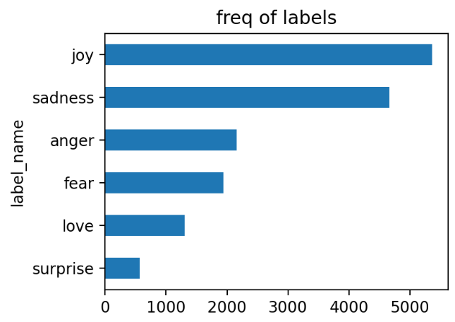
Data Data Load - emotions 这里选择使用emotions数据集,常用于文本情感分类,识别句子或段落中表达的情感类别,包括6类标签(sadness, joy, love, anger, fear, surprise)。
1
2
from datasets import load_dataset
emotions = load_dataset ( "emotions" )
通过打印emotions可以看到emotions数据集的组成,共有两万条数据,$Size_{Train} : Size_{Vali} : Size_{Test} = 8 : 1 : 1$,每个数据有text和label两个features(dict of dict):
 1
 2
 3
 4
 5
 6
 7
 8
 9
10
11
12
13
14
DatasetDict({
    train: Dataset({
        features: ['text', 'label'],
        num_rows: 16000
    })
    validation: Dataset({
        features: ['text', 'label'],
        num_rows: 2000
    })
    test: Dataset({
        features: ['text', 'label'],
        num_rows: 2000
    })
})
labels = emotions['train'].features['label'].names可以查看各个标签。
Data Visualization Analysis 简单可视化分析一下数据集,主要任务有:
1
2
3
4
# Task 1: dataset -> dataframe
emotions_df = pd . DataFrame . from_dict ( emotions [ 'train' ]) # 取出训练集
emotions_df [ 'label_name' ] = emotions_df [ 'label' ] . apply ( lambda x : labels [ x ]) # 加入标签名列
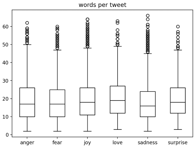
emotions_df [ 'words per tweet' ] = emotions_df [ 'text' ] . str . split () . apply ( len ) # 统计words数
接下来可以简单分析:
1
2
3
4
5
6
7
# 统计标签数
emotions_df . label . value_counts ()
emotions_df . label_name . value_counts ()
# 查看最长/短文本
emotions_df [ 'words per tweet' ] . max ()
emotions_df [ 'words per tweet' ] . idxmax ()
emotions_df . iloc [ ... ][ 'text' ]
简单的可视化:
 1
 2
 3
 4
 5
 6
 7
 8
 9
10
11
# Labels' Freq
plt . figure ( figsize = ( 4 , 3 ))
emotions_df [ 'label_name' ] . value_counts ( ascending = True ) . plot . barh ()
plt . title ( 'freq of labels' )
# Words / Tweet
plt . figure ( figsize = ( 4 , 3 ))
emotions_df [ 'words per tweet' ] = emotions_df [ 'text' ] . str . split () . apply ( len ) # 简单统计
emotions_df . boxplot ( 'words per tweet' , by = 'label_name' ,
showfliers = True , grid = False , color = 'black' )
plt . suptitle ( '' )
plt . xlabel ( '' )
标签频率 文本长度
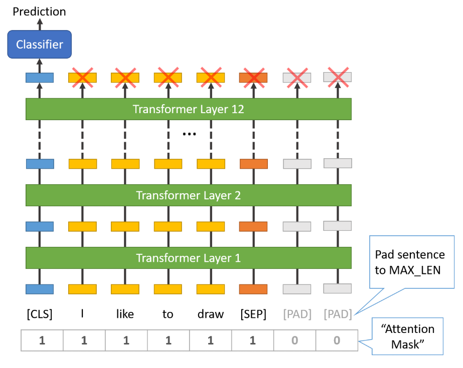
Text2Tokens 为了后续模型的训练,需要将数据集转换为模型接受的输入类型。对于model,需要关注BERT/DistillBERT使用subword tokenizer;对于tokenizer,需要关注tokenizer.vocab_size、model_max_length和model_input_name几个参数。
 1
 2
 3
 4
 5
 6
 7
 8
 9
10
11
12
13
14
15
from transformers import AutoTokenizer
model_ckpt = "/path/to/bert-distill"
tokenizer = AutoTokenizer . from_pretrained ( model_ckpt )
print ( tokenizer . vocab_size , tokenizer . model_max_length , tokenizer . model_input_names )
# 30522 512 ['input_ids', 'attention_mask']
# 输出一个batch的text, 输出一个batch的tokens
def batch_tokenize ( batch ):
return tokenizer ( batch [ 'text' ], padding = True , truncation = True )
emotions_encoded = emotions . map ( batch_tokenize , batched = True , batch_size = None )
# type(emotions_encoded['train']['input_ids'][0]) == list
# list to tensor
emotions_encoded . set_format ( 'torch' , columns = [ 'input_ids' , 'attention_mask' , 'label' ])
Model Fine-Tuning Load Model DistillBERT-base-uncased是huggingface提供的一个轻量级BERT模型,由知识蒸馏(Knowledge Distillation)技术训练,在保持高性能的同时大幅减少了模型参数,使推理速度更快、计算资源需求更低。
1
2
3
from transformers import AutoModel
model_ckpt = '/home/HPC_ASC/bert-distill'
model = AutoModel . from_pretrained ( model_ckpt )
通过model可以发现,相较于BERT baseline,这个蒸馏后的模型在Embedding Layer减少了token_type_embedding(只有word embedding和position embedding),将原本12层Transformer Layer改为6层。
1
2
3
4
5
6
def get_params ( model ):
model_parameters = filter ( lambda p : p . requires_grad , model . parameters ())
params = sum ([ np . prod ( p . size ()) for p in model_parameters ])
return params
get_params ( model ) # return np.int64(66362880) 相较于bert-base-uncased少了约40%参数
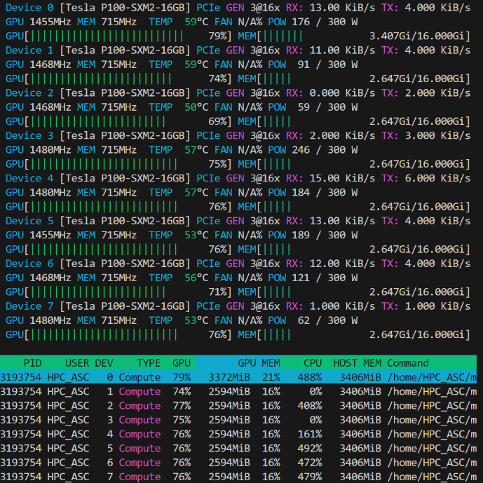
接下来加载模型,可以通过nvidia-smi或nvtop(如果正确安装和配置了的话)可以看到加载到显存中的模型占用约546MiB。
1
2
3
4
from transformers import AutoModelForSequenceClassification # 和AutoModel不同,后者没有分类头 -> 下游任务
modle_ckpt = '/home/HPC_ASC/distilbert-base-uncased'
device = torch . device ( 'cuda' if torch . cuda . is_available () else 'cpu' )
model = AutoModelForSequenceClassification . from_pretrained ( model_ckpt , num_labels = num_classes , ignore_mismatched_sizes = True ) . to ( device )
我们需要导入并定义huggingface提供的训练API来完成高效的模型训练。在正式定义Trainer前,还需要一个辅助函数来确定Trainer的参数指标:
 1
 2
 3
 4
 5
 6
 7
 8
 9
10
def compute_classification_metrics ( pred ):
# pred: PredictionOutput, from trainer.predict(dataset)
# true label
labels = pred . label_ids
# pred
preds = pred . predictions . argmax ( - 1 )
f1 = f1_score ( labels , preds , average = "weighted" )
acc = accuracy_score ( labels , preds )
precision = precision_score ( labels , preds , average = "macro" )
return { "accuracy" : acc , "f1" : f1 , "precision" : precision }
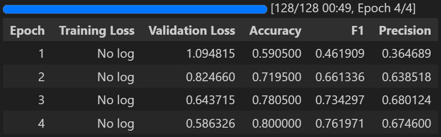
接下来正式定义Trainer(在这一步可能会提示你需要安装transformers[torch]或accelerator >= 0.26?,务必不要直接pip install transformers[torch],这会导致卸载我本地已安装的torch (v2.7.0)并安装torch (v2.6.0),从而让torchvision等包的版本不匹配,进而引发更多错误),并开始模型训练:
 1
 2
 3
 4
 5
 6
 7
 8
 9
10
11
12
13
14
15
16
17
18
19
20
21
22
23
24
25
26
27
# https://huggingface.co/docs/transformers/main_classes/trainer
from transformers import TrainingArguments , Trainer
batch_size = 64
logging_steps = len ( emotions_encoded [ 'train' ]) // batch_size # 160,000 // batch_size
model_name = f ' { model_ckpt } _emotion_ft_0531'
training_args = TrainingArguments ( output_dir = model_name ,
num_train_epochs = 4 ,
learning_rate = 2e-5 ,
weight_decay = 0.01 , # 默认使用AdamW的优化算法
per_device_train_batch_size = batch_size ,
per_device_eval_batch_size = batch_size ,
eval_strategy = "epoch" ,
disable_tqdm = False ,
logging_steps = logging_steps ,
# write
push_to_hub = True ,
log_level = "error" )
trainer = Trainer ( model = model ,
tokenizer = tokenizer ,
train_dataset = emotions_encoded [ 'train' ],
eval_dataset = emotions_encoded [ 'validation' ],
args = training_args ,
compute_metrics = compute_classification_metrics )
trainer . train ()
nvtop: 硬件环境是一机八卡Tesla P100 16G Model Training 训练好的模型权重会存放在当前目录的model_name(bert-distill_emotion_ft_0531)下。
Inference 1
2
3
4
5
6
7
8
9
10
11
12
13
14
preds_output = trainer . predict ( emotions_encoded [ 'test' ])
y_preds = np . argmax ( preds_output . predictions , axis =- 1 )
y_true = emotions_encoded [ 'validation' ][ 'label' ]
# for classification
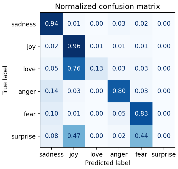
def plot_confusion_matrix ( y_preds , y_true , labels ):
cm = confusion_matrix ( y_true , y_preds , normalize = "true" )
fig , ax = plt . subplots ( figsize = ( 4 , 4 ))
disp = ConfusionMatrixDisplay ( confusion_matrix = cm , display_labels = labels )
disp . plot ( cmap = "Blues" , values_format = ".2f" , ax = ax , colorbar = False )
plt . title ( "Normalized confusion matrix" )
plot_confusion_matrix ( y_preds , y_true , labels )
Confusion Matrix 可以写一个辅助函数,将测试集的loss和预测结果映射到测试集中:
 1
 2
 3
 4
 5
 6
 7
 8
 9
10
11
12
13
14
15
16
17
18
from torch.nn.functional import cross_entropy
def forward_pass_with_label ( batch ):
# Place all input tensors on the same device as the model
inputs = { k : v . to ( device ) for k , v in batch . items ()
if k in tokenizer . model_input_names }
with torch . no_grad ():
output = model ( ** inputs )
pred_label = torch . argmax ( output . logits , axis =- 1 )
loss = cross_entropy ( output . logits , batch [ 'label' ] . to ( device ),
reduction = 'none' )
# Place outputs on CPU for compatibility with other dataset columns
return { "loss" : loss . cpu () . numpy (),
"predicted_label" : pred_label . cpu () . numpy ()}
emotions_encoded [ 'validation' ] = emotions_encoded [ 'validation' ] . map (
forward_pass_with_label , batched = True , batch_size = 16
)
Push into Huggingface 1
2
3
4
5
6
# 在Jupyter Jotebook中登录huggingface
# 需要在huggingface注册一个writable token
from huggingface_hub import notebook_login
notebook_login ()
trainer . push_to_hub ( commit_message = "Training completed!" )
Huggingface Login Huggingface Repo Page 当需要在其他地方调用这个模型时,可以通过transformers包的pipeline轻松实现:
1
2
3
4
5
6
7
from transformers import pipeline
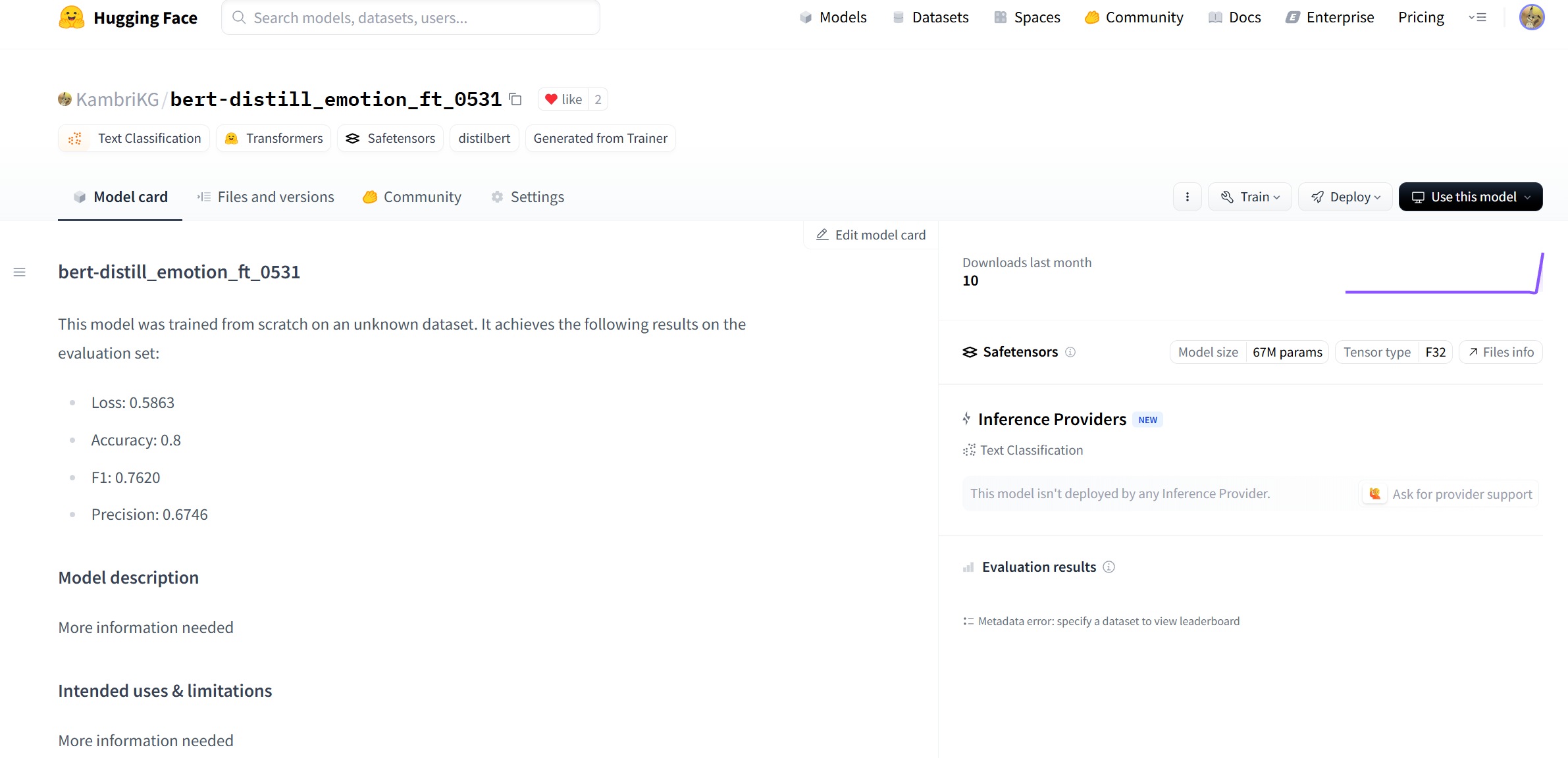
model_id = "KambriKG/bert-distill_emotion_ft_0531"
classifier = pipeline ( "text-classification" , model = model_id )
custom_tweet = "I saw a movie today and it was really good"
preds = classifier ( custom_tweet , return_all_scores = True )
Reference BERT: Pre-training of Deep Bidirectional Transformers for Language Understanding
Huggingface-BERT文档
Chris McCormick’s Blog
动手学深度学习(PyTorch)
bilibili-五道口纳什-BERT、T5、GPT合集
学习BERT时在五道口纳什的频道收益良多,《动手写BERT》系列教程非常适合对LLM有一定认识但缺乏实践经验的入门者学习参考。